How to Calculate OEE: Formula, Worked Example, and Python Code

Overall Equipment Effectiveness (OEE) is the most widely used metric for answering one simple question: of the time we planned to make good parts, how much did we actually spend making good parts at full speed?

It is also one of the most misunderstood. Two plants can report "75% OEE" and mean completely different things. This guide walks through the formula, a full worked example, the losses behind each factor, a Python implementation, and how to collect the data automatically from your machines.

What OEE measures

OEE compares what a machine or line actually produced against what it could have produced in the time it was scheduled to run. A score of 100% means only good parts, as fast as possible, with no stops.

It is built from three factors, each capturing a different kind of loss:

• Availability: was the machine running when it was supposed to?
• Performance: when it was running, was it running at full speed?
• Quality: of what it made, how much was good the first time?

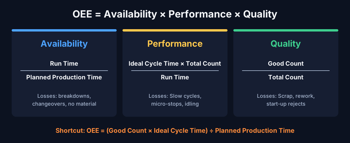
Because the factors multiply, small losses compound. 90% × 90% × 90% is only 72.9%.

The data you need

Before calculating anything, collect five numbers for the period you are measuring (a shift, a day, a production order):

• Planned Production Time: total time minus planned non-production time such as breaks, scheduled maintenance or no orders. Example: 450 min
• Stop Time: time the machine was scheduled but not running, such as breakdowns, changeovers or waiting for material. Example: 45 min
• Ideal Cycle Time: the fastest time to produce one part under ideal conditions. Example: 1.2 s
• Total Count: every part produced, good or bad. Example: 17,500
• Good Count: parts that passed quality the first time, with no rework. Example: 17,150

Step-by-step: a worked example

Let's take one 8-hour shift on a packaging line.

Step 1: Planned Production Time

The shift is 480 minutes. There are two 15-minute breaks, which are planned stops.

Planned Production Time = 480 − 30 = 450 min

Step 2: Availability

During the shift the line had a 25-minute breakdown and a 20-minute changeover: 45 minutes of stops.

Run Time = 450 − 45 = 405 min

Availability = Run Time ÷ Planned Production Time = 405 ÷ 450 = 90.0%

Step 3: Performance

The ideal cycle time is 1.2 seconds per part (50 parts per minute). In 405 minutes of running, the line made 17,500 parts.

Performance = (Ideal Cycle Time × Total Count) ÷ Run Time

= (1.2 s × 17,500) ÷ (405 × 60 s) = 21,000 ÷ 24,300 = 86.4%

At full speed, the line could have made 20,250 parts in that run time. It made 17,500. The gap comes from slow cycles and short stops that never got logged as downtime.

Step 4: Quality

Of the 17,500 parts, 350 were rejected.

Good Count = 17,500 − 350 = 17,150

Quality = Good Count ÷ Total Count = 17,150 ÷ 17,500 = 98.0%

Step 5: OEE

OEE = 90.0% × 86.4% × 98.0% = 76.2%

Check it with the shortcut

There is a simpler formula that gives the same answer and is a good sanity check:

OEE = (Good Count × Ideal Cycle Time) ÷ Planned Production Time

= (17,150 × 1.2 s) ÷ (450 × 60 s) = 20,580 ÷ 27,000 = 76.2%

The shortcut tells you the score. The three factors tell you where the losses are, which is what you need to improve it.

Seeing OEE as time

Another way to read OEE is as a waterfall of time. Start from planned production time and subtract each loss:

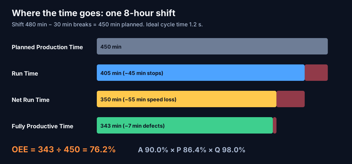
• Availability loss: 45 minutes the line was stopped.
• Performance loss: 55 minutes worth of production lost to running slower than ideal (405 min run time − 350 min of ideal-speed production).
• Quality loss: 7 minutes spent making 350 parts that were scrapped.

What remains, 343 minutes, is Fully Productive Time: the time spent making only good parts, at full speed, with no stops. 343 ÷ 450 = 76.2%.

This view is useful in meetings: "we lost 55 minutes to speed this shift" is easier to act on than "performance was 86%".

The Six Big Losses

Each OEE factor maps to two of the classic Six Big Losses from Total Productive Maintenance (TPM):

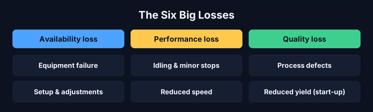
Availability losses

• Equipment failure: breakdowns, tooling failures, unplanned maintenance
• Setup and adjustments: changeovers, material shortages, warm-up

Performance losses

• Idling and minor stops: jams, misfeeds, blocked or starved conveyors, sensor faults
• Reduced speed: running below nameplate, worn equipment, inconsistent operation

Quality losses

• Process defects: scrap and rework during stable production
• Reduced yield: scrap during start-up or after a changeover

A practical decision: where does a short stop count? Many plants set a threshold, for example stops under 2 minutes count as performance loss (minor stops) and anything longer as availability loss (downtime). Pick one, document it, and keep it consistent.

What is a good OEE score?

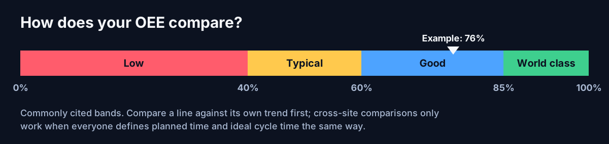
These bands are commonly cited:

• 100%: perfect production. Rarely a realistic target.
• 85%: often called "world class" for discrete manufacturing, based on roughly 90% availability, 95% performance and 99.9% quality.
• 60%: fairly typical for discrete manufacturers, with substantial room to improve.
• 40%: low, and common when companies first start measuring.

Treat these as rough guides, not targets. A batch process, a high-mix job shop and a single-product bottling line will have very different realistic ceilings. The most useful comparison is a line against its own history, measured the same way every time.

Common mistakes that distort OEE

1. Using a "standard" cycle time instead of the ideal one. If you use the average or the budgeted rate, performance will look close to 100% and hide the speed losses. Use the fastest cycle the machine can sustain, usually the nameplate rate or the best demonstrated rate.

2. Performance above 100%. This almost always means the ideal cycle time is wrong, or the part counter is double-counting. Fix the input, don't cap the result.

3. Excluding changeovers from planned time. Changeovers are a loss you can reduce (see SMED). If you treat them as planned downtime, you hide one of the biggest improvement opportunities.

4. Counting rework as good. Quality should count only parts that were right the first time.

5. Averaging OEE across lines. Taking the simple mean of three lines' OEE gives a wrong number when they ran for different amounts of time. Aggregate correctly instead:

Plant OEE = Σ Fully Productive Time ÷ Σ Planned Production Time

or equivalently, sum good count × ideal cycle time across lines, then divide by the total planned time.

6. Manual data on a clipboard. Handwritten logs systematically miss short stops and slow cycles, so performance comes out too high. That is the main argument for automatic data collection.

OEE vs. TEEP

OEE measures how well you use the time you planned to run. TEEP (Total Effective Equipment Performance) measures how well you use all the time on the calendar:

TEEP = OEE × Utilization

Utilization = Planned Production Time ÷ All Time

If our example line runs only that one 450-minute shift per day:

Utilization = 450 ÷ 1,440 = 31.3%

TEEP = 76.2% × 31.3% = 23.8%

OEE tells you how well you run the line. TEEP tells you how much capacity you have before you need to buy another one.

Calculating OEE in Python

Here is a minimal, dependency-free implementation of the worked example:

from dataclasses import dataclass


@dataclass
class ShiftData:
    planned_time_s: float      # planned production time, seconds
    stop_time_s: float         # unplanned + changeover stops, seconds
    ideal_cycle_time_s: float  # fastest sustainable time per part, seconds
    total_count: int           # every part produced, good or bad
    good_count: int            # parts that passed first time


def oee(d: ShiftData) -> dict:
    run_time = d.planned_time_s - d.stop_time_s
    availability = run_time / d.planned_time_s
    performance = (d.ideal_cycle_time_s * d.total_count) / run_time
    quality = d.good_count / d.total_count
    return {
        "availability": availability,
        "performance": performance,
        "quality": quality,
        "oee": availability * performance * quality,
    }


shift = ShiftData(
    planned_time_s=450 * 60,
    stop_time_s=45 * 60,
    ideal_cycle_time_s=1.2,
    total_count=17_500,
    good_count=17_150,
)

for k, v in oee(shift).items():
    print(f"{k:>12}: {v:6.1%}")

Output:

availability:  90.0%
 performance:  86.4%
     quality:  98.0%
         oee:  76.2%

In production you would add guards for division by zero (a shift with no planned time or no parts), keep the ideal cycle time per product rather than per machine, and store the raw inputs alongside the result so you can recalculate when definitions change.

Collecting OEE data automatically with IIoT

OEE is only as good as its inputs. In an IIoT architecture, the data typically comes from four places:

• Machine state (running, stopped, faulted, idle): PLC tags read via OPC UA, Modbus or a native driver
• Total count and reject count: PLC counters, vision systems, checkweighers
• Ideal cycle time per product: MES, ERP routing, or a product master table
• Planned production time: shift calendar and production schedule from MES or ERP

A common pattern:

1. Edge layer: a gateway or SCADA platform reads state and counters from the PLC, timestamps them and publishes changes to an MQTT broker.
2. Unified Namespace (UNS): the data is organized by plant hierarchy, for example site/area/line/machine/state, so any application can subscribe to it.
3. Contextualization: the current product, order and shift are attached so each count knows its ideal cycle time and each stop knows whether it was planned.
4. Calculation: a service computes Availability, Performance and Quality continuously, usually in rolling windows (current hour, current shift, last 24 hours), and writes the results back to the UNS and to a historian.
5. Visualization: dashboards show the live OEE, the loss waterfall and a Pareto of stop reasons.

Two practical tips:

• Capture stop reasons at the source. A state change from "running" to "stopped" is only half the story. Pair it with a reason code, either from the PLC's alarm logic or from a quick operator selection on an HMI, so you can build a downtime Pareto.
• Count from the machine, not the report. The difference between the PLC counter and the end-of-shift paperwork is often the first improvement opportunity you find.

Key takeaways

• OEE = Availability × Performance × Quality, or simply good count × ideal cycle time ÷ planned production time.
• The factors matter more than the score: they tell you whether to work on downtime, speed or defects.
• Use the true ideal cycle time and don't hide changeovers in planned downtime.
• Aggregate with time-weighted sums, never with simple averages.
• Compare lines against their own trend, using consistent definitions.
• Automate data collection. Manual logs miss exactly the small losses OEE is designed to expose.

If you work on OEE systems, MES or IIoT data pipelines, this is one of the most in-demand skill sets in manufacturing today. Browse current openings on IIoTjob.